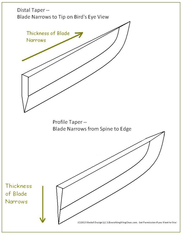
Hereby goes blade with a box (arb8) on top, intersected with with an arb6
intersected with the other arb6, that makes the bottom of the blade sharp.
the Distal Taper.
Mario.
Post by Mario MeissnerSean,
thank you for the extensive explanation, and sorry for the
misunderstanding. When you said that "instead of considering the ray line
lets consider segments" I thought that these segments were something else
not related to the rays. Let me attempt to summarize everything into a
bullet-list, see if things start getting clearer. I'll try to be specific,
and there probably will be mistakes but that's intentional as I want to
make sure I understand everything well before moving on. Please correct me
on anything inaccurate or wrong.
- During ray-tracing, the calling code prepares the application and
ray-tracing instance and shoots rays at the geometry. The library code
containing the hit, miss and other functions handles the information it
receives when a ray hits geometry.
- The hit function receives a set of partitions in a circular linked
list, (taken from the example:) "each [partition] describing one in
and out segment of one region for each region encountered". So each
partition is basically a set of segments, and all partitions together tell
us all the stuff the ray went through. I assume there are many different
"partitions" because we put the segments of different regions in different
partitions, but also partitions can have more than one segment because we
can cross a region more than once with a ray.
- In rtweight specifically, each ray gets fired some distance away
from the other rays, in a grid. Thus we can think of the rays as a square
tube, that has 2mm side length for the square and goes through the geometry
(I assume these are the "cells" that appear in the code of viewweight.c)
All the volume captured inside will be handled by one call of the hit
function. Looping through all the partitions and obtaining the volume we
crossed, and the density assigned to the region, we compute the mass for
each partition and store it in some data structure (which seems to be this
"datapoint" thing). Finally we just need to add it all up and obtain our
total mass.
- In order to support heterogeneous densities we need a representation
that allows us to provide the necessary information to the hit function,
who will query our representation to obtain the density of the in and out
points, and possibly the rate of change between the two. We then
integrate/interpolate to obtain the "average" density of our segment, so
that we can continue the same way we did in the point above.
- I guess the biggest "difficulty" here is to define a proper way of
telling the hit function what this rate of change between the points is.
Also storing a proper definition of the material density that allows for
this information to be queried easily. This is why storing functions and
taking derivatives is not a good idea. Instead we may want to store vectors
that tell the rate of change in several directions. Density at a specific
point could be retrieved by combining vectors and the rate of change
between two arbitrary points can be obtained through the vectors as well.
Will send new blade soon.
Mario.
Post by Mario MeissnerOkay, so let's make sure I understand the current code before
continuing with the new specifications.
Post by Mario MeissnerAbout the blade, yes I tried to just mix both because that made it
simpler.
Post by Mario MeissnerTomorrow I'll make the new blade (without the curve) and get going with
the code. It seems like I'm missing some basic concepts on what's going on
inside. I'll try to understand it as good as I can and then ask some
questions on what isn't clear to me. Is there any documentation on what
exactly happens during geometry evaluation and ray tracing in general?
http://brlcad.org/wiki/Example_Application
For the abstract conceptual concepts of ray tracing, anything that talks
about âsolidâ or âfull pathâ ray tracing is generally relevant (as opposed
to ray tracing for image synthesis, rendering pictures). Coincidentally
relevant: http://slideplayer.com/slide/9271245/
What usually gets in the way are preconceptions. Consider for example an
object, some unknown object. You donât (yet) know what it looks like, how
big it is, etc. All you have is a special ray/gun that shoots an
infinitely thin ray through the object and tells you when you entered and
shoot entry exit
o-> ray . . . . . hit oâ-âââo hit
6mm
All you know at this point is that you hit it and 6mm later, the ray
exited the object. That by itself isnât very useful, but we can shoot a
whole set of rays, each from a different position, and we start to get a
o-> ray1 oâo
o-> ray2 oâââââo
oâ> ray3 oâââââââââo
o-> ray4 oâââââââââââââo
oâ> ray5 oâââââââââo
o-> ray6 oâââââo
o-> ray7 oâo
We start to see it looks a bit like a rotated cube. Moreover, knowing
the length of each segment and the spacing of the rays, we could actually
o-> ray1 oâo 2mm
o-> ray2 oâââââo 6mm
oâ> ray3 oâââââââââo 10mm
o-> ray4 oâââââââââââââo 14mm
oâ> ray5 oâââââââââo 10mm
o-> ray6 oâââââo 6mm
o-> ray7 oâo 2mm
ââââ
with 2mm spacing between rays: 50mm x 2mm = 100mm^2 area
Itâs probably a 10mm x 10mm square. Extend that example into layer after
layer of samples and you donât just have an area estimate, but now you have
a (3D) volume estimate because each ray represents a 2D cross section
with 2mm spacing between rays: 50mm x 2mm x 2mm = 200mm^3 volume
With a volume estimate and knowing density, you can obviously calculate
mass too (mass = volume x density). And all of that was done without
knowing anything about the geometry. Thatâs essentially what rtweight is
doing.
With your project, weâre changing the last step. In mathematical terms,
we were doing a summation over all the individual volume bits, multiplying
each by a constant density. New form, everything stays the same except
weâre either going to multiply the volume by a different (e.g., average)
density based on a function or weâre going to further parameterize the
volume so an volume/mass integral can be estimated.
Cheers!
Sean
------------------------------------------------------------
------------------
Check out the vibrant tech community on one of the world's most
engaging tech sites, Slashdot.org! http://sdm.link/slashdot
_______________________________________________
BRL-CAD Developer mailing list
https://lists.sourceforge.net/lists/listinfo/brlcad-devel